FVGP Single Task Notebook

In this notebook we will go through a few features of fvGP. We will be primarily concerned with regression over a single dimension output and single task. See the multiple_task_test_notebook.ipynb for single dimension and multiple task example. The extension to multiple dimensions is straight forward.

Import fvgp and relevant libraries

import fvgp
from fvgp import gp
import numpy as np
import matplotlib.pyplot as plt

Defining some input data and testing points

def function(x):
    return np.sin(1.1 * x)+np.cos(0.5 * x)
x_data = np.linspace(-2*np.pi, 10*np.pi,50).reshape(-1,1)
y_data = function(x_data)
x_pred = np.linspace(-2*np.pi, 10 * np.pi, 1000)

Setting up the fvgp single task object

NOTE: The input data need to be given in the form (N x input_space_dim). The output can either be a N array or N x 1 array where N is the number of data points. See help(gp.GP) for more information.

obj = gp.GP(1, x_data,y_data, init_hyperparameters = np.array([10,10]),use_inv = False)

Training our gaussian process regression on given data

hyper_param_bounds = np.array([[0.001, 5.],[ 0.001, 100]])
##this will block the main thread, even if you use "hgdl", another option is "global" or "local"
obj.train(hyper_param_bounds, method = "hgdl")

/home/docs/checkouts/readthedocs.org/user_builds/fvgp/envs/stable/lib/python3.8/site-packages/distributed/dashboard/core.py:20: UserWarning: 
Dask needs bokeh >= 2.4.2, < 3 for the dashboard.
You have bokeh==3.1.0.
Continuing without the dashboard.
  warnings.warn(

/home/docs/checkouts/readthedocs.org/user_builds/fvgp/envs/stable/lib/python3.8/site-packages/scipy/optimize/_minimize.py:554: RuntimeWarning: Method L-BFGS-B does not use Hessian information (hess).
  warn('Method %s does not use Hessian information (hess).' % method,

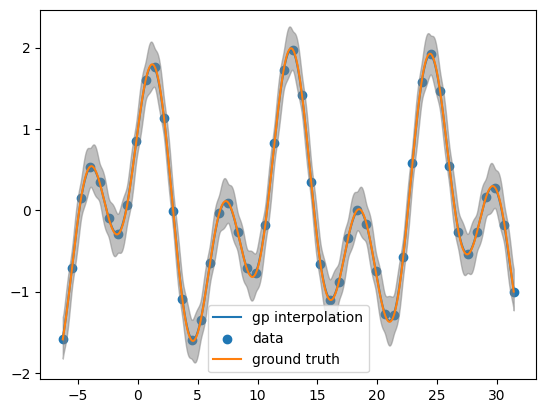
Looking the posterior mean at the test points

post_mean= obj.posterior_mean(x_pred.reshape(-1,1))["f(x)"]
post_var= obj.posterior_covariance(x_pred.reshape(-1,1))["v(x)"]

plt.plot(x_pred, post_mean, label='gp interpolation')
plt.scatter(x_data, y_data, label='data')
plt.plot(x_pred,function(x_pred), label = 'ground truth')
plt.fill_between(x_pred, post_mean + 3.0 *np.sqrt(post_var),post_mean - 3.0 * np.sqrt(post_var), color = 'grey', alpha = 0.5)
plt.legend()

<matplotlib.legend.Legend at 0x7f133220a3d0>

Training Asynchronously

obj = gp.GP(1, x_data,y_data, init_hyperparameters = np.array([10,10]),
                            variances = np.zeros(y_data.reshape(-1,1).shape))

hyper_param_bounds = np.array([[0.0001, 100], [ 0.0001, 100]])

async_obj = obj.train_async(hyper_param_bounds)

/home/docs/checkouts/readthedocs.org/user_builds/fvgp/envs/stable/lib/python3.8/site-packages/distributed/dashboard/core.py:20: UserWarning: 
Dask needs bokeh >= 2.4.2, < 3 for the dashboard.
You have bokeh==3.1.0.
Continuing without the dashboard.
  warnings.warn(

Updating asynchronously

Updates hyperparameters to current optimization values

obj.update_hyperparameters(async_obj)

array([10, 10])

Killing training

obj.kill_training(async_obj)

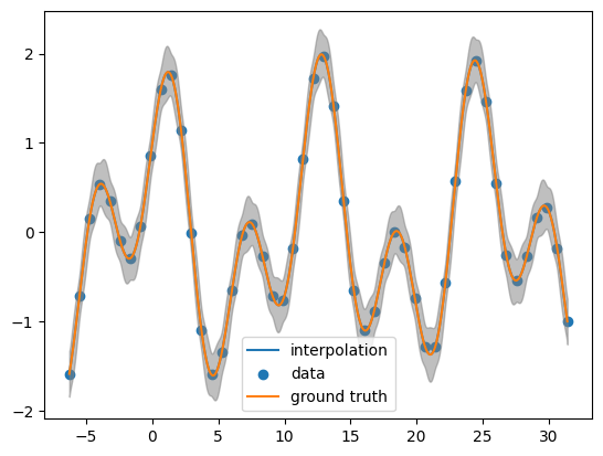
Looking at the posterior mean at the test points

post_mean= obj.posterior_mean(x_pred.reshape(-1,1))['f(x)']

plt.plot(x_pred, post_mean, label='interpolation')
plt.scatter(x_data, y_data, label='data')
plt.plot(x_pred, function(x_pred), label='ground truth')
plt.fill_between(x_pred, post_mean + 3.0 *np.sqrt(post_var),post_mean - 3.0 * np.sqrt(post_var), color = 'grey', alpha = 0.5)
plt.legend()

<matplotlib.legend.Legend at 0x7f13dfc71e50>

Custom Kernels

def kernel_l1(x1,x2, hp, obj):
    ################################################################
    ###standard anisotropic kernel in an input space with l1########
    ################################################################
    d1 = abs(np.subtract.outer(x1[:,0],x2[:,0])) 
    return hp[0] * np.exp(-d1/hp[1])

obj = gp.GP(1, x_data,y_data,
                init_hyperparameters = np.array([10,10]),
                variances = np.zeros(y_data.shape),
                gp_kernel_function = kernel_l1)

Training our gaussian process regression on given data

hyper_param_bounds = np.array([[0.0001, 1000],[ 0.0001, 1000]])
obj.train(hyper_param_bounds)

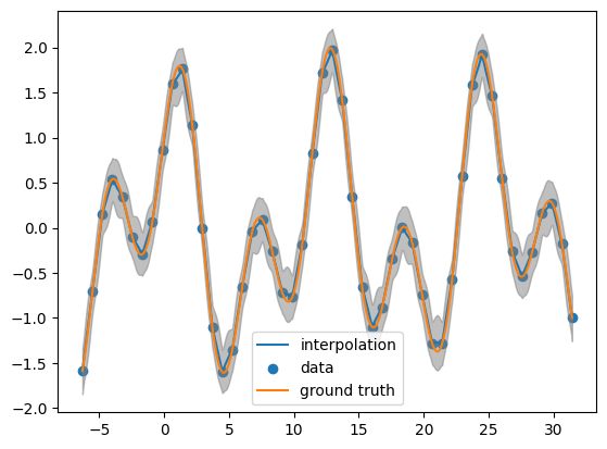
Looking the posterior mean at the test points

post_mean= obj.posterior_mean(x_pred.reshape(-1,1))["f(x)"]

plt.plot(x_pred, post_mean, label='interpolation')
plt.scatter(x_data, y_data, label='data')
plt.plot(x_pred, function(x_pred), label='ground truth')
plt.fill_between(x_pred, post_mean + 3.0 *np.sqrt(post_var),post_mean - 3.0 * np.sqrt(post_var), color = 'grey', alpha = 0.5)
plt.legend()

<matplotlib.legend.Legend at 0x7f13dfb921f0>

Prior Mean Functions

NOTE: The prior mean function must return a 1d vector, e.g., (100,)

def example_mean(x,hyperparameters,gp_obj):
    return np.ones(len(x))

obj = gp.GP(1, x_data,y_data,init_hyperparameters = np.array([10,10]),
                            variances = np.zeros(y_data.shape),
                            gp_mean_function = example_mean)

Training our gaussian process regression on given data

hyper_param_bounds = np.array([[0.0001, 1000],[ 0.0001, 1000]])
obj.train(hyper_param_bounds)

Looking the posterior mean at the test points

post_mean= obj.posterior_mean(x_pred.reshape(-1,1))["f(x)"]

plt.plot(x_pred, post_mean, label='interpolation')
plt.scatter(x_data, y_data, label='data')
plt.plot(x_pred, function(x_pred), label='ground truth')
plt.fill_between(x_pred, post_mean + 3.0 *np.sqrt(post_var),post_mean - 3.0 * np.sqrt(post_var), color = 'grey', alpha = 0.5)
plt.legend()

<matplotlib.legend.Legend at 0x7f13dfab6550>