Single-Task Test#
#install the right fvgp version
#!pip install fvgp~=4.8.0
Setup#
import numpy as np
import matplotlib.pyplot as plt
from fvgp import GP
import time
from distributed import Client
client = Client()

%load_ext autoreload
%autoreload 2
from itertools import product
x_pred1D = np.linspace(0,1,1000).reshape(-1,1)
Data#
x = np.linspace(0,600,1000)
def f1(x):
return np.sin(5. * x) + np.cos(10. * x) + (2.* (x-0.4)**2) * np.cos(100. * x)
#np.random.seed(42)
x_data = np.random.rand(200).reshape(-1,1)
y_data = f1(x_data[:,0]) + (np.random.rand(len(x_data))-0.5) * 0.5
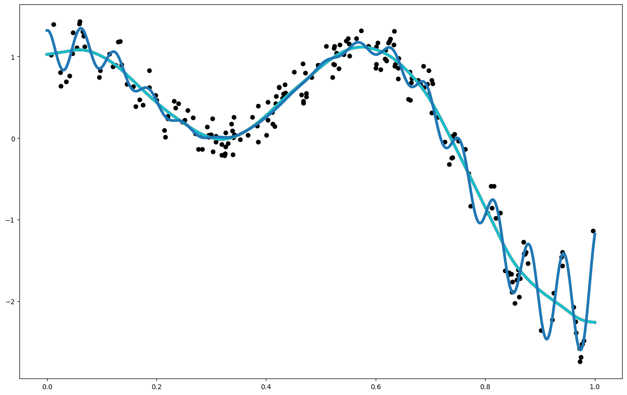
plt.figure(figsize = (15,5))
plt.xticks([0.,0.5,1.0])
plt.yticks([-2,-1,0.,1])
plt.xticks(fontsize=20)
plt.yticks(fontsize=20)
plt.plot(x_pred1D,f1(x_pred1D), color = 'orange', linewidth = 4)
plt.scatter(x_data[:,0],y_data, color = 'black')
<matplotlib.collections.PathCollection at 0x7f676442d750>
Customizing a Gaussian Process#
from fvgp.kernels import *
from scipy import sparse
def my_noise(x,hps):
    #This is a simple noise function, but can be arbitrarily complex using many hyperparameters.
    #The noise can be a vector, a matrix, or a sparse matrix in case gp2Scale is used.
    return np.zeros(len(x)) + hps[2]

#stationary
def skernel(x1,x2,hps):
    #The kernel follows the mathematical definition of a kernel. This
    #means there is no limit to the variety of kernels you can define.
    d = get_distance_matrix(x1,x2)
    return hps[0] * matern_kernel_diff1(d,hps[1])


def meanf(x, hps):
    #This ios a simple mean function but it can be arbitrarily complex using many hyperparameters.
    return np.sin(hps[3] * x[:,0])

#it is a good idea to plot the prior mean function to make sure we did not mess up
plt.figure(figsize = (15,5))
plt.plot(x_pred1D,meanf(x_pred1D, np.array([1.,1.,5.0,2.])), color = 'orange', label = 'task1')
[<matplotlib.lines.Line2D at 0x7f67640d1050>]
Initialization and different training options#
st = time.time()
from loguru import logger
logger.disable("fvgp")
my_gp1 = GP(x_data,y_data,
            init_hyperparameters = np.ones((4))*10.,  # we need enough of those for kernel, noise, and prior mean functions
            noise_variances=np.ones(y_data.shape) * 0.01, # providing noise variances and a noise function will raise a warning
            compute_device='cpu',
            kernel_function=skernel,
            kernel_function_grad=None,
            prior_mean_function=meanf,
            prior_mean_function_grad=None,
            #noise_function=my_noise,
            gp2Scale = False,
            linalg_mode='Inv',
            ram_economy=True,
            )


hps_bounds = np.array([[0.01,100.], #signal variance for the kernel
                       [0.01,100.], #length scale for the kernel
                       [0.001,0.1],  #noise
                       [0.01,1.]  #mean
                      ])

#the following is not needed, this is just to show how data is replced or appended
x_update = np.array([0.1,0.2,0.5]).reshape(3,1)
y_update = f1(x_update[:,0]) + (np.random.rand(len(x_update))-0.5) * 0.5
my_gp1.update_gp_data(x_update,
                      y_update,
                      noise_variances_new=np.ones(y_update.shape) * 0.05,
                      append=True, rank_n_update=True)


print("Standard Training (MCMC)")
hps = my_gp1.train(hyperparameter_bounds=hps_bounds, info = False)
print("Result=", hps, "after ", time.time() - st, " seconds")
print("ML: ",my_gp1.log_likelihood())
print("")

print("ADAM")
hps = my_gp1.train(hyperparameter_bounds=hps_bounds, info = True, max_iter = 100, method="adam")
print("Result=", hps, "after ", time.time() - st, " seconds")
print("ML: ",my_gp1.log_likelihood())
print("")

print("Global Training")
hps = my_gp1.train(hyperparameter_bounds=hps_bounds, method='global', max_iter = 20)
print("Result=", hps, "after ", time.time() - st, " seconds")
print("ML: ",my_gp1.log_likelihood())
print("")

print("Local Training")
hps = my_gp1.train(hyperparameter_bounds=hps_bounds, method='local')
print("Result=", hps, "after ", time.time() - st, " seconds")
print("ML: ",my_gp1.log_likelihood())
print("")

print("HGDL Training")
hps = my_gp1.train(hyperparameter_bounds=hps_bounds, method='hgdl', max_iter=2, dask_client=client)
print("Result=", hps, "after ", time.time() - st, " seconds")
print("ML: ",my_gp1.log_likelihood())
print("")
Standard Training (MCMC)
Result= [9.86917135e+01 3.09074818e-01 8.59776600e-03 8.11258426e-01] after  10.545368671417236  seconds
ML:  -24.104609033919445

ADAM
Result= [9.79240104e+01 2.79840110e-01 8.59776600e-03 7.38042777e-01] after  12.5807523727417  seconds
ML:  -23.206988762840552

Global Training
Result= [1.08970257 0.05567086 0.03447922 0.24807967] after  21.208317041397095  seconds
ML:  -8.137923631944176

Local Training
Result= [0.90112351 0.05154835 0.03447922 0.01      ] after  22.306291341781616  seconds
ML:  -7.558800665386229

HGDL Training
Result= [0.89924315 0.05149113 0.03447922 0.01      ] after  37.08134937286377  seconds
ML:  -7.558773583289195
#You can always test your gradient like this before running local optimizers
my_gp1.test_log_likelihood_gradient(np.array([1.,1.,1.,1.]), epsilon=1e-6)
(array([  82.88698348, -223.52898225,    0.        ,   -1.77303662]),
 array([  82.88696924, -223.52898043,   -0.        ,   -1.77303804]))
More advanced: Asynchronous training#
Train asynchronously – via Adam, HGDL, or MCMC – on a remote server or locally. You can also start a bunch of different training runs on different computers. This training will continue without any signs of life until you query the solution via ‘update_hyperparameters(object)’ or call ‘my_gp1.stop_training(opt_obj)’
HGDL#
my_gp1.set_hyperparameters(np.array([1.,1.,1.,1.]))
print(my_gp1.hyperparameters)
opt_obj = my_gp1.train(hyperparameter_bounds=hps_bounds, dask_client=client, asynchronous=True, method='hgdl')
# The result won't change much (or at all) since this is such a simple optimization
for i in range(20):
    my_gp1.update_hyperparameters(opt_obj)
    print("iteration ", i, " : ",my_gp1.hyperparameters)
    time.sleep(0.1)
my_gp1.stop_training(opt_obj) ##this leaves the dask client alive, kill_client() will shut it down.
[1. 1. 1. 1.]
iteration  0  :  [1. 1. 1. 1.]
/home/marcus/Coding/fvGP/fvgp/gp.py:880: UserWarning: Hyperparameter update not successful len(optima list) = 0
  hps = self.trainer.update_hyperparameters(opt_obj)
iteration  1  :  [1. 1. 1. 1.]
iteration  2  :  [1. 1. 1. 1.]
iteration  3  :  [1. 1. 1. 1.]
iteration  4  :  [1. 1. 1. 1.]
iteration  5  :  [1. 1. 1. 1.]
iteration  6  :  [1. 1. 1. 1.]
iteration  7  :  [0.89924229 0.0514911  0.01536715 0.01      ]
iteration  8  :  [0.89924229 0.0514911  0.01536715 0.01      ]
iteration  9  :  [0.89924229 0.0514911  0.01536715 0.01      ]
iteration  10  :  [0.89924229 0.0514911  0.01536715 0.01      ]
iteration  11  :  [0.89924229 0.0514911  0.01536715 0.01      ]
iteration  12  :  [0.89924229 0.0514911  0.01536715 0.01      ]
iteration  13  :  [0.89924229 0.0514911  0.01536715 0.01      ]
iteration  14  :  [0.89924229 0.0514911  0.01536715 0.01      ]
iteration  15  :  [0.89924229 0.0514911  0.01536715 0.01      ]
iteration  16  :  [0.89924229 0.0514911  0.01536715 0.01      ]
iteration  17  :  [0.89924229 0.0514911  0.01536715 0.01      ]
iteration  18  :  [0.89924229 0.0514911  0.01536715 0.01      ]
iteration  19  :  [0.89924229 0.0514911  0.01536715 0.01      ]
ADAM#
my_gp1.set_hyperparameters(np.array([1.,1.,1.,1.]))
print(my_gp1.hyperparameters)
opt_obj = my_gp1.train(hyperparameter_bounds=hps_bounds, dask_client=client, asynchronous=True, method='adam')
# The result won't change much (or at all) since this is such a simple optimization
for i in range(20):
    my_gp1.update_hyperparameters(opt_obj)
    print("iteration ", i, " : ",my_gp1.hyperparameters)
    time.sleep(0.1)
my_gp1.stop_training(opt_obj) ##this leaves the dask client alive, kill_client() will shut it down.
[1. 1. 1. 1.]
iteration  0  :  [2.19715846e+01 5.89966475e+01 3.12846742e-02 1.66248991e-01]
iteration  1  :  [2.20315527e+01 5.89366788e+01 3.12846742e-02 1.06177319e-01]
iteration  2  :  [2.21212219e+01 5.88469172e+01 3.12846742e-02 1.56037736e-02]
iteration  3  :  [ 2.22396195e+01  5.87279558e+01  3.12846742e-02 -1.04501090e-01]
iteration  4  :  [ 2.23657347e+01  5.86000750e+01  3.12846742e-02 -2.26564473e-01]
iteration  5  :  [ 2.24326675e+01  5.85316650e+01  3.12846742e-02 -2.84362283e-01]
iteration  6  :  [ 2.25556443e+01  5.84052926e+01  3.12846742e-02 -3.67624398e-01]
iteration  7  :  [ 2.26681266e+01  5.82888943e+01  3.12846742e-02 -4.10813995e-01]
iteration  8  :  [ 2.27522682e+01  5.82013473e+01  3.12846742e-02 -4.23737372e-01]
iteration  9  :  [ 2.28835158e+01  5.80645231e+01  3.12846742e-02 -4.23378270e-01]
iteration  10  :  [ 2.30155743e+01  5.79263601e+01  3.12846742e-02 -4.15070411e-01]
iteration  11  :  [ 2.31105674e+01  5.78268196e+01  3.12846742e-02 -4.10420095e-01]
iteration  12  :  [ 2.32156478e+01  5.77163348e+01  3.12846742e-02 -4.07680917e-01]
iteration  13  :  [ 2.32443400e+01  5.76860945e+01  3.12846742e-02 -4.07266691e-01]
iteration  14  :  [ 2.33305372e+01  5.75949717e+01  3.12846742e-02 -4.06489752e-01]
iteration  15  :  [ 2.34265792e+01  5.74932437e+01  3.12846742e-02 -4.05898060e-01]
iteration  16  :  [ 2.34554135e+01  5.74626572e+01  3.12846742e-02 -4.05700481e-01]
iteration  17  :  [ 2.34842439e+01  5.74320177e+01  3.12846742e-02 -4.05481001e-01]
iteration  18  :  [ 2.36093705e+01  5.72989870e+01  3.12846742e-02 -4.04257586e-01]
iteration  19  :  [ 2.36866013e+01  5.72166982e+01  3.12846742e-02 -4.03342822e-01]
MCMC#
my_gp1.set_hyperparameters(np.array([1.,1.,1.,1.]))
print(my_gp1.hyperparameters)
opt_obj = my_gp1.train(hyperparameter_bounds=hps_bounds, dask_client=client, asynchronous=True, method='mcmc')
# The result won't change much (or at all) since this is such a simple optimization
for i in range(20):
    my_gp1.update_hyperparameters(opt_obj)
    print("iteration ", i, " : ",my_gp1.hyperparameters)
    time.sleep(0.1)
my_gp1.stop_training(opt_obj) ##this leaves the dask client alive, kill_client() will shut it down.
[1. 1. 1. 1.]
iteration  0  :  [1. 1. 1. 1.]
iteration  1  :  [35.34583355 32.60746749  0.06289679  0.41558595]
iteration  2  :  [21.09837953  0.19594692  0.0712251   0.40831958]
iteration  3  :  [21.09837953  0.19594692  0.0712251   0.40831958]
iteration  4  :  [22.26667251  0.16665617  0.06875945  0.42502987]
iteration  5  :  [20.88801971  0.16918544  0.06944989  0.43228463]
iteration  6  :  [20.88801971  0.16918544  0.06944989  0.43228463]
iteration  7  :  [21.00338036  0.18623     0.06968631  0.44066631]
iteration  8  :  [21.00338036  0.18623     0.06968631  0.44066631]
iteration  9  :  [21.16688864  0.16869511  0.06971167  0.44256742]
iteration  10  :  [21.16688864  0.16869511  0.06971167  0.44256742]
iteration  11  :  [21.16688864  0.16869511  0.06971167  0.44256742]
iteration  12  :  [21.16688864  0.16869511  0.06971167  0.44256742]
iteration  13  :  [20.39673407  0.14922826  0.0701446   0.44413563]
iteration  14  :  [20.39673407  0.14922826  0.0701446   0.44413563]
iteration  15  :  [20.756826    0.17578913  0.06960743  0.44292018]
iteration  16  :  [20.756826    0.17578913  0.06960743  0.44292018]
iteration  17  :  [21.60291036  0.17451937  0.06978896  0.4389262 ]
iteration  18  :  [21.60291036  0.17451937  0.06978896  0.4389262 ]
iteration  19  :  [21.60291036  0.17451937  0.06978896  0.4389262 ]
The Result#
#let's make a prediction
x_pred = np.linspace(0,1,1000)
hps = my_gp1.train(hyperparameter_bounds=hps_bounds, info = False)
# different ways to call
var1 = my_gp1.posterior_covariance(x_pred.reshape(-1,1), variance_only=False, add_noise=False)["v(x)"]
var1 = my_gp1.posterior_covariance(x_pred.reshape(-1,1), variance_only=False, add_noise=True)["v(x)"]
mean1 = my_gp1.posterior_mean(x_pred.reshape(-1,1))["m(x)"]
var1 = my_gp1.posterior_covariance(x_pred.reshape(-1,1), variance_only=False, add_noise=True)["v(x)"]
mean_grad = my_gp1.posterior_mean_grad(x_pred.reshape(-1,1), direction=0)["dm/dx"]
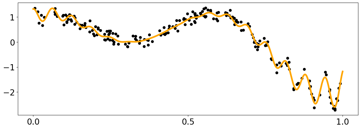
print("Posterior Mean and Uncertainty")
plt.figure(figsize = (16,10))
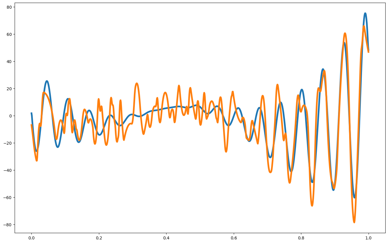
plt.plot(x_pred,mean1, label = "posterior mean", linewidth = 4)
plt.plot(x_pred1D,f1(x_pred1D), label = "latent function", linewidth = 4)
plt.fill_between(x_pred, mean1 - 3. * np.sqrt(var1), mean1 + 3. * np.sqrt(var1), alpha = 0.5, color = "grey", label = "var")
plt.scatter(my_gp1.x_data,my_gp1.y_data, color = 'black')
plt.show()
print("Posterior Mean Gradient")
plt.figure(figsize = (16,10))
dx = 1./len(x_pred)
plt.plot(x_pred1D,np.gradient(f1(x_pred1D).flatten(), dx), label = "ground truth gradient", linewidth = 4)
plt.plot(x_pred1D,mean_grad, label = "posterior mean grad", linewidth = 4)
plt.show()
##looking at some validation metrics
print("RMSE: ",my_gp1.rmse(x_pred1D,f1(x_pred1D).flatten()))
print("NRMSE: ",my_gp1.nrmse(x_pred1D,f1(x_pred1D).flatten()))
print("CRPS (mean, std): ",my_gp1.crps(x_pred1D,f1(x_pred1D).flatten()))
print("R2: ",my_gp1.r2(x_pred1D,f1(x_pred1D).flatten()))
print("NLPD: ",my_gp1.nlpd(x_pred1D,f1(x_pred1D).flatten()))
print("MSLL: ",my_gp1.msll(x_pred1D,f1(x_pred1D).flatten()))
print("MAPE: ",my_gp1.mape(x_pred1D,f1(x_pred1D).flatten()))
print("INTERVAL SCORE: ",my_gp1.interval_score(x_pred1D,f1(x_pred1D).flatten()))
print("MPIW: ",my_gp1.mpiw(x_pred1D))
print("PICP: ",my_gp1.picp(x_pred1D,f1(x_pred1D).flatten()))
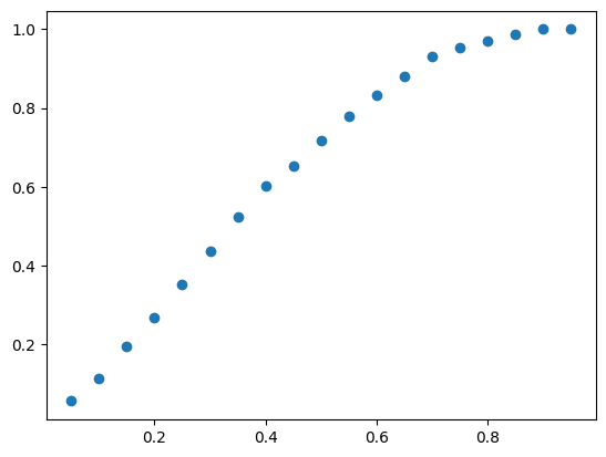
print("Coverage Curve:")
cov_curve = my_gp1.coverage_curve(x_pred1D,f1(x_pred1D).flatten())
plt.scatter(cov_curve["target_coverage"], cov_curve["measured_coverage"])
plt.show()
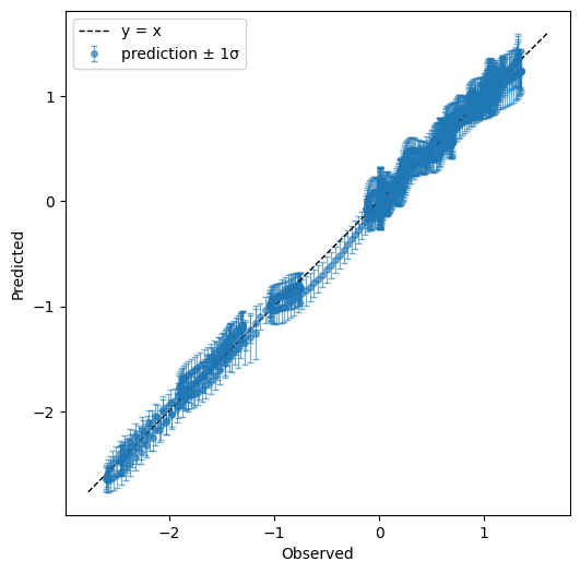
print("predicted vs. observed")
my_gp1.plot_observed_vs_predicted(x_pred1D,f1(x_pred1D).flatten())
Posterior Mean and Uncertainty
Posterior Mean Gradient
RMSE:              0.07770443001481848
NRMSE:             0.019702412788305618
CRPS (mean, std):  (np.float64(0.04529064240060971), np.float64(0.02917160166184701))
R2:                0.9943287143467242
NLPD:              -1.0892162663212972
MSLL:              -2.542310644617157
MAPE:              1.0281077220832522
INTERVAL SCORE:    0.5128672744378368
MPIW:              0.5128672744378368
PICP:              1.0
Coverage Curve:
predicted vs. observed
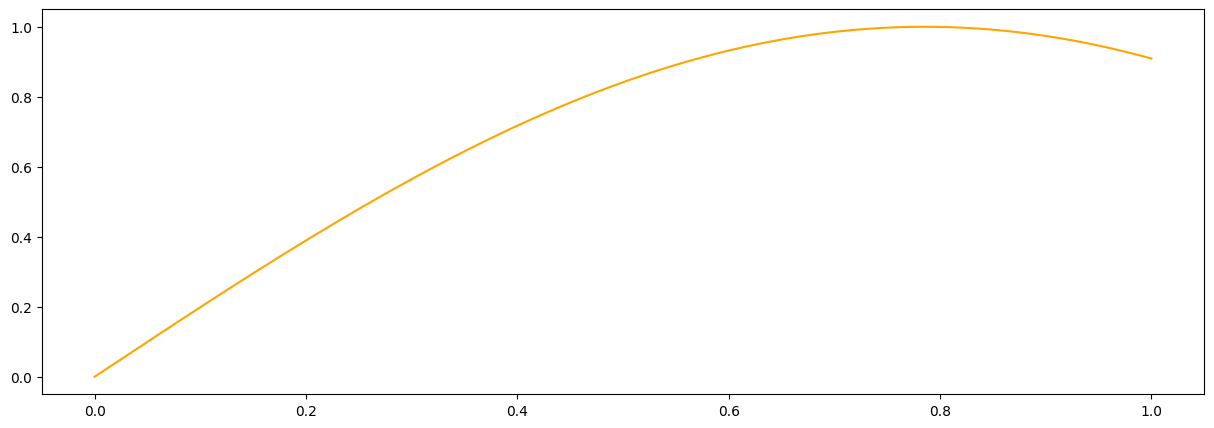
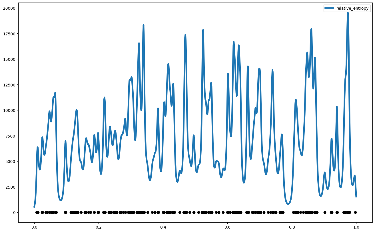
Predicted Information Gain#
relative_entropy = my_gp1.gp_relative_information_entropy_set(x_pred.reshape(-1,1))["RIE"]
plt.figure(figsize = (16,10))
plt.plot(x_pred,relative_entropy, label = "relative_entropy", linewidth = 4)
plt.scatter(x_data,y_data, color = 'black')
plt.legend()
<matplotlib.legend.Legend at 0x7f69fc5fbf10>
#We can ask mutual information and total correlation there is given some test data
x_test = np.array([[0.45],[0.45]])
print("MI: ",my_gp1.gp_mutual_information(x_test))
print("TC: ",my_gp1.gp_total_correlation(x_test))
my_gp1.gp_entropy(x_test)
my_gp1.gp_entropy_grad(x_test, 0)
my_gp1.gp_kl_div(x_test, np.ones((len(x_test))), np.identity((len(x_test))))
my_gp1.gp_relative_information_entropy(x_test)
my_gp1.gp_relative_information_entropy_set(x_test)
my_gp1.posterior_covariance(x_test)
my_gp1.posterior_covariance_grad(x_test)
my_gp1.posterior_mean(x_test)
my_gp1.posterior_mean_grad(x_test)
my_gp1.posterior_probability(x_test, np.ones((len(x_test))), np.identity((len(x_test))))
MI:  {'x': array([[0.45],
       [0.45]]), 'mutual information': np.float64(6.115516079637928)}
TC:  {'x': array([[0.45],
       [0.45]]), 'total correlation': np.float64(18.17934238219496)}
{'mu': array([0.76067907, 0.76067907]),
 'covariance': array([[0.01804132, 0.00756118],
        [0.00756118, 0.01804132]]),
 'probability': np.float64(0.1473577208467523)}
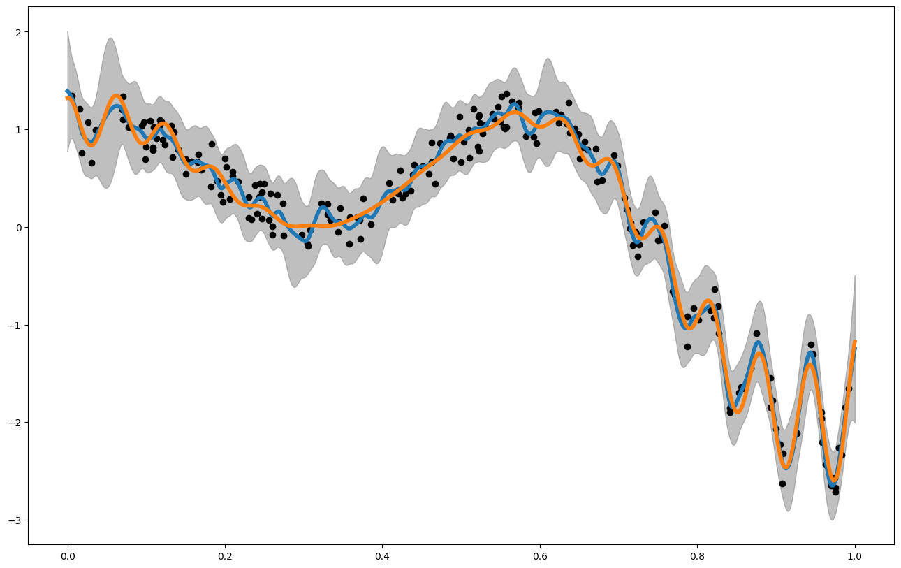
Running many GPs at once in parallel#
#duplicate data: in practice, this would be different data in every column
y_data = np.broadcast_to(y_data[:, None], (y_data.size, 10))

my_gp1 = GP(x_data,y_data,
            init_hyperparameters = np.ones((2))/10.,  # we need enough of those for kernel, noise, and prior mean functions
            noise_variances=np.ones(y_data.shape[0]) * 0.1, # providing noise variances and a noise function will raise a warning
            compute_device='cpu',
            )


hps_bounds = np.array([[0.01,10.], #signal variance for the kernel
                       [0.01,10.], #length scale for the kernel
                      ])

print("Standard Training (MCMC)")
hps = my_gp1.train(hyperparameter_bounds=hps_bounds, info = True, max_iter = 100)
print("Result=", hps, "after ", time.time() - st, " seconds")
print("")
Standard Training (MCMC)
Starting likelihood. f(x)=  -60.530918611011415
Finished  10  out of  100  iterations. f(x)=  -34.55797599219602
Finished  20  out of  100  iterations. f(x)=  -34.55797599219602
Finished  30  out of  100  iterations. f(x)=  -35.549605153076385
Finished  40  out of  100  iterations. f(x)=  -32.24174967992212
Finished  50  out of  100  iterations. f(x)=  -33.68759856747093
Finished  60  out of  100  iterations. f(x)=  -32.918954595562866
Finished  70  out of  100  iterations. f(x)=  -33.10616455337518
Finished  80  out of  100  iterations. f(x)=  -33.501944176110385
Finished  90  out of  100  iterations. f(x)=  -32.80656151215575
Result= [4.55115124 0.5521299 ] after  68.61876678466797  seconds
x_pred = np.linspace(0,1,1000).reshape(1000,1)
mean = my_gp1.posterior_mean(x_pred)["m(x)"]
sd   = np.sqrt(my_gp1.posterior_covariance(x_pred)["v(x)"])
print("Posterior Means")
plt.figure(figsize = (16,10))
for i in range(10):
    plt.plot(x_pred.flatten(),mean[:,i], label = "posterior mean", linewidth = 4)
plt.scatter(my_gp1.x_data,my_gp1.y_data[:,0], color = 'black')
plt.plot(x_pred1D,f1(x_pred1D), label = "latent function", linewidth = 4)
plt.show()
Posterior Means