gp2Scale#
gp2Scale is a special setting in fvgp that combines non-stationary, compactly-supported kernels, HPC distributed computing, and sparse linear algebra to allow scale-up of exact GPs to millions of data points. gp2Scale holds the world record in this category! Here we run a moderately-sized GP, just because we assume you might run this locally.
I hope it is clear how cool it is what is happening here. If you have a dask client that points to a remote cluster with 500 GPUs, you will distribute the covariance matrix computation across those. The full matrix is sparse and will be fast to work with in downstream operations. The algorithm only makes use of naturally-occuring sparsity, so the result is exact in contrast to Vecchia or inducing-point methods.
##first install the newest version of fvgp
#!pip install fvgp~=4.8.0
#!pip install imate
Setup#
import numpy as np
import matplotlib.pyplot as plt
from fvgp import GP
from dask.distributed import Client
import sys
%load_ext autoreload
%autoreload 2

#further control plotting
from loguru import logger
logger.disable("fvgp")


client = Client() ##this is the client you can make locally like this or
#your HPC team can provide a script to get it. We included an example to get gp2Scale going
#on Perlmutter


#It's good practice to make sure to wait for all the workers to be ready
client.wait_for_workers(4)
Preparing the data and some other inputs#
def f1(x):
    return ((np.sin(5. * x) + np.cos(10. * x) + (2.* (x-0.4)**2) * np.cos(100. * x)))

input_dim = 1
N = 2000
x_data = np.random.rand(N,input_dim)
y_data = f1(x_data).reshape(len(x_data))
hps_n = 2

hps_bounds = np.array([[0.1,1.],      ##signal var of Wendland kernel
                       [0.001,0.04]])  ##length scale for Wendland kernel
Standard MCMC training#
from fvgp.kernels import wendland_anisotropic_gp2Scale_cpu
def kernel(x1,x2,hps):
    return wendland_anisotropic_gp2Scale_cpu(x1,x2,hps)


init_hps = np.array([0.2, 0.02])
my_gp2S = GP(x_data,y_data, kernel_function=kernel,
             init_hyperparameters = init_hps, #compute_device = 'gpu', #you can use gpus here
             gp2Scale = True, gp2Scale_batch_size= 1000,
             dask_client = client, linalg_mode = "Chol")

#optional data update
x_update = np.random.rand(5,input_dim)
y_update = f1(x_update).reshape(len(x_update))
my_gp2S.update_gp_data(x_update, y_update, append = True, rank_n_update = True)


my_gp2S.train(hyperparameter_bounds = hps_bounds, max_iter = 100, info=True)
Starting likelihood. f(x)=  5848.578741395031
Finished  10  out of  100  iterations. f(x)=  6007.324839312315
Finished  20  out of  100  iterations. f(x)=  6126.330421201296
Finished  30  out of  100  iterations. f(x)=  6310.268868945442
Finished  40  out of  100  iterations. f(x)=  6379.971930057959
Finished  50  out of  100  iterations. f(x)=  6531.830835892909
Finished  60  out of  100  iterations. f(x)=  6534.654215764308
Finished  70  out of  100  iterations. f(x)=  6570.242257876666
Finished  80  out of  100  iterations. f(x)=  6576.950098377039
Finished  90  out of  100  iterations. f(x)=  6599.066659784158
array([0.20138893, 0.03948361])
A custom MCMC#
from fvgp import ProposalDistribution
init_s = (np.diag(hps_bounds[:,1]-hps_bounds[:,0])/100.)**2


def obj_func(hps,args):
    return my_gp2S.log_likelihood(hyperparameters=hps[0:2])

from fvgp import gpMCMC
def proposal_distribution(x0, hps, obj):
    cov = obj.prop_args["prop_Sigma"]
    proposal_hps = np.zeros((len(x0)))
    proposal_hps = np.random.multivariate_normal(
        mean = x0, cov = cov, size = 1).reshape(len(x0))
    return proposal_hps

def in_bounds(v,bounds):
    if any(v<bounds[:,0]) or any(v>bounds[:,1]): return False
    return True

def prior_function(theta,bounds,args):
    if in_bounds(theta, bounds):
        return 0.
    else:
        return -np.inf

pd = ProposalDistribution([0,1] ,proposal_dist=proposal_distribution,
                        init_prop_Sigma = init_s, adapt_callable="normal")

my_mcmc = gpMCMC(obj_func, bounds=hps_bounds, prior_function=prior_function, proposal_distributions=[pd],)
logger.disable("fvgp")
hps = np.random.uniform(
                        low = hps_bounds[:,0],
                        high = hps_bounds[:,1],
                        size = len(hps_bounds))
mcmc_result = my_mcmc.run_mcmc(x0=hps, n_updates=110, break_condition="default", info = True)

my_gp2S.set_hyperparameters(mcmc_result["x"][-1])
Starting likelihood. f(x)=  6363.353783872716
Finished  10  out of  110  iterations. f(x)=  6414.230962180892
Finished  20  out of  110  iterations. f(x)=  6460.482380152246
Finished  30  out of  110  iterations. f(x)=  6464.734926258102
Finished  40  out of  110  iterations. f(x)=  6464.734926258102
Finished  50  out of  110  iterations. f(x)=  6471.523579203583
Finished  60  out of  110  iterations. f(x)=  6472.7143721053135
Finished  70  out of  110  iterations. f(x)=  6479.888436307762
Finished  80  out of  110  iterations. f(x)=  6479.176589153875
Finished  90  out of  110  iterations. f(x)=  6480.19890618533
Finished  100  out of  110  iterations. f(x)=  6482.374845420839
Posterior evaluation#
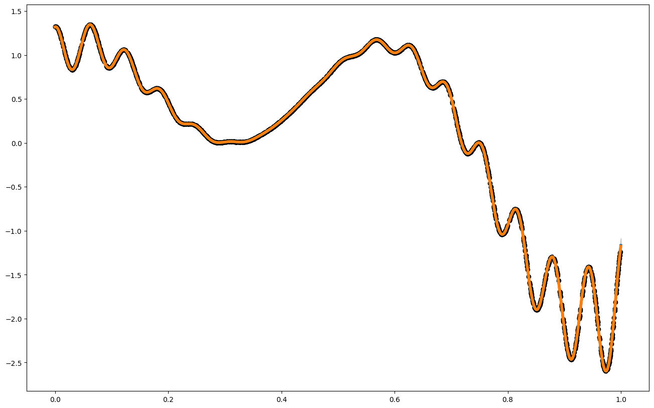
x_pred = np.linspace(0,1,1000) ##for big GPs, this is usually not a good idea, but in 1d, we can still do it
                               ##It's better to do predictions only for a handful of points at a time.

mean1 = my_gp2S.posterior_mean(x_pred.reshape(1000,1))["m(x)"]
var1 =  my_gp2S.posterior_covariance(x_pred.reshape(1000,1), variance_only=False)["v(x)"]


plt.figure(figsize = (16,10))
plt.plot(x_pred,mean1, label = "posterior mean", linewidth = 4)
plt.plot(x_pred,f1(x_pred), label = "latent function", linewidth = 4)
plt.fill_between(x_pred, mean1 - 3. * np.sqrt(var1), mean1 + 3. * np.sqrt(var1), alpha = 0.5, color = "grey", label = "var")
plt.scatter(x_data,y_data, color = 'black')
<matplotlib.collections.PathCollection at 0x7fad9c68fc10>