GGMP — 1D Distributional Regression Demo

This notebook demonstrates the Gaussian GP for Gaussian Mixture data (GGMP) model on a synthetic 1D example.

Each “observation” at an input location \(x\) is not a scalar but an entire probability distribution. The true generating process is a two-component Gaussian mixture whose component means vary smoothly with \(x\):

\[p(y \mid x) = w_1 \, \mathcal{N}\!\left(y \mid \mu_1(x),\, \sigma_1^2\right) + w_2 \, \mathcal{N}\!\left(y \mid \mu_2(x),\, \sigma_2^2\right)\]

with \(\mu_1(x) = -1.0 + 0.6\sin(2\pi x)\) (always negative) and \(\mu_2(x) = 1.5 + 0.5\cos(\pi x)\) (always positive). The two modes never cross, which keeps component identification trivial via sort-by-mean.

The GGMP workflow has three phases (per the GGMP paper):

1. Local GMM fitting — fit a K-component GMM at each station to extract per-component means and variances; align components across stations.

2. Component-wise GP training — one GP per component, trained on the aligned component means with the per-component variances as the noise.

3. Mixture weight optimization — EM on the density objective.

Stages 2 and 3 are both performed by GGMP.train(). Stage 1 we do explicitly below so that initLikelihoods() receives meaningful per-component means and variances. Skipping Stage 1 and relying on the default initialization causes the GPs to collapse to constants, because the default uses the bimodal variance (which is huge) as the GP noise.

CAUTION: Beta release. The current implementation of GGMP is a proof-of-concept and may contain unknown bugs.
It is recommended to test on synthetic data before applying to real datasets.

import numpy as np
import matplotlib.pyplot as plt
from scipy.stats import norm

from fvgp import ggmp as ggmp_module
from fvgp.ggmp import GGMP, hyperparameters, fit_gmm_fixed_weights

rng = np.random.default_rng(42)

plt.rcParams.update({
    "figure.dpi": 130,
    "font.size": 11,
    "axes.spines.top": False,
    "axes.spines.right": False,
})
BLUE, ORANGE, GREEN, RED = "#3A86FF", "#FF6B35", "#2EC4B6", "#E63946"

1. Synthetic data

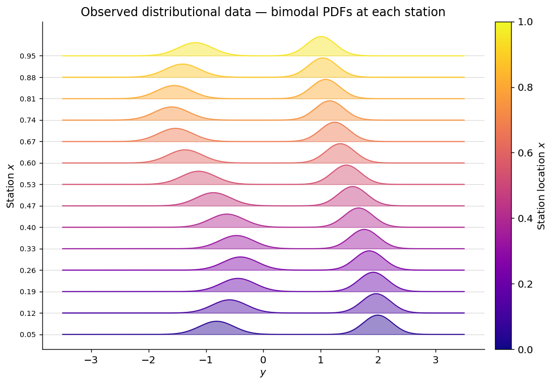
We place 14 training stations in \([0.05, 0.95]\). At each station we draw 500 samples from the true two-component GMM and store both the samples (for Stage 1 GMM fitting) and a smoothed density curve (the y_data GGMP expects).

# True generating process.  Non-crossing component means keep sort-by-mean
# alignment correct across stations.
K = 2
w_true = np.array([0.45, 0.55])
sigma1, sigma2 = 0.30, 0.25

def mu1(x):
    """Lower mode: always in [-1.6, -0.4]."""
    return np.squeeze(-1.0 + 0.6 * np.sin(2 * np.pi * np.asarray(x, dtype=float).ravel()))

def mu2(x):
    """Upper mode: always in [1.0, 2.0]."""
    return np.squeeze( 1.5 + 0.5 * np.cos(np.pi     * np.asarray(x, dtype=float).ravel()))

N_train = 14
x_train = np.linspace(0.05, 0.95, N_train).reshape(-1, 1)
domain  = np.linspace(-3.5, 3.5, 300)

n_samples_per_station = 500
y_data = []
station_samples = []
for xi in x_train[:, 0]:
    m1, m2 = float(mu1(xi)), float(mu2(xi))

    # Sample from the true GMM at this station
    comp = rng.choice(2, size=n_samples_per_station, p=w_true)
    samp = np.where(comp == 0,
                    rng.normal(m1, sigma1, n_samples_per_station),
                    rng.normal(m2, sigma2, n_samples_per_station))
    station_samples.append(samp)

    # Smooth density on a shared grid (this is what y_data must contain)
    dens = (w_true[0] * norm.pdf(domain, m1, sigma1) +
            w_true[1] * norm.pdf(domain, m2, sigma2))
    y_data.append((domain.copy(), dens))

N_pred = 120
x_pred = np.linspace(0.0, 1.0, N_pred).reshape(-1, 1)

print(f"Generated {N_train} stations × {n_samples_per_station} samples each.")

Generated 14 stations × 500 samples each.

Plot: observed distributional data

Each ridge is one station’s smoothed PDF — clearly bimodal because the two modes are always well-separated.

fig, ax = plt.subplots(figsize=(9, 6))
cmap = plt.cm.plasma
offset_scale = 1.5

for i, (xi, (dom, dens)) in enumerate(zip(x_train[:, 0], y_data)):
    offset = i * offset_scale
    norm_dens = dens / (dens.max() + 1e-12) * offset_scale * 0.9
    color = cmap(xi)
    ax.fill_between(dom, offset, offset + norm_dens, alpha=0.45, color=color)
    ax.plot(dom, offset + norm_dens, lw=1.0, color=color)
    ax.axhline(offset, color="#cccccc", lw=0.5, zorder=0)

sm = plt.cm.ScalarMappable(cmap=cmap, norm=plt.Normalize(0, 1))
sm.set_array([])
cb = fig.colorbar(sm, ax=ax, pad=0.02)
cb.set_label("Station location $x$")

ax.set_xlabel("$y$")
ax.set_yticks(np.arange(N_train) * offset_scale)
ax.set_yticklabels([f"{xi:.2f}" for xi in x_train[:, 0]], fontsize=8)
ax.set_ylabel("Station $x$")
ax.set_title("Observed distributional data — bimodal PDFs at each station")
plt.tight_layout(); plt.show()

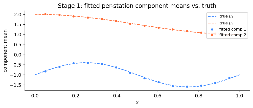
2. Phase 1 — local GMM fitting

For each station we fit a \(K=2\) GMM to its samples using fit_gmm_fixed_weights (a 1D EM fitter that returns components sorted by mean). Because \(\mu_1(x) < \mu_2(x)\) at every \(x\), sorting trivially aligns components — no Hungarian step needed.

The fitted per-station, per-component variances become the GP noise. This is the key difference from the default initialization (which would use the much larger bimodal variance).

fitted_means = np.zeros((K, N_train))
fitted_vars  = np.zeros((K, N_train))

for n, samples in enumerate(station_samples):
    means_n, vars_n = fit_gmm_fixed_weights(samples, K, w_true, max_iter=80)
    fitted_means[:, n] = means_n   # already sorted by mean
    fitted_vars[:, n]  = vars_n

print("Phase-1 GMM fit quality:")
for k in range(K):
    true_mu  = mu1(x_train) if k == 0 else mu2(x_train)
    true_var = sigma1**2  if k == 0 else sigma2**2
    mae_mu  = np.mean(np.abs(fitted_means[k] - true_mu))
    mae_var = np.mean(np.abs(fitted_vars[k] - true_var))
    print(f"  Component {k+1}: MAE(mean)={mae_mu:.3f}  MAE(var)={mae_var:.4f}")

# Visual check of Stage 1
fig, ax = plt.subplots(figsize=(8, 3.5))
xx = np.linspace(0, 1, 200)
ax.plot(xx, mu1(xx), "--", color=BLUE,   lw=1.5, label=r"true $\mu_1$")
ax.plot(xx, mu2(xx), "--", color=ORANGE, lw=1.5, label=r"true $\mu_2$")
ax.scatter(x_train[:, 0], fitted_means[0], color=BLUE,   s=35, edgecolors="white",
           label="fitted comp 1", zorder=5)
ax.scatter(x_train[:, 0], fitted_means[1], color=ORANGE, s=35, edgecolors="white",
           label="fitted comp 2", zorder=5)
ax.set_xlabel("$x$"); ax.set_ylabel("component mean")
ax.set_title("Stage 1: fitted per-station component means vs. truth")
ax.legend(fontsize=9, loc="upper right")
plt.tight_layout(); plt.show()

Phase-1 GMM fit quality:
  Component 1: MAE(mean)=0.017  MAE(var)=0.0066
  Component 2: MAE(mean)=0.011  MAE(var)=0.0042

3. Build the GGMP model

Each component GP uses a Matérn kernel with three hyperparameters: signal variance, length scale, and a trainable constant prior mean. We pass the Stage-1 fitted means and standard deviations into initLikelihoods so each component GP sees the right signal and a realistic (small) noise level.

# 3 params per GP: [signal_var, length_scale, prior_mean]
hps_init   = [np.array([0.3, 0.3, 0.0])] * K
hps_bounds = [np.array([[0.01, 5.0],
                         [0.05, 3.0],
                         [-5.0, 5.0]])] * K

weights_init   = np.ones(K) / K
weights_bounds = np.array([[0.01, 1.0]] * K)

hps_obj = hyperparameters(weights_init, weights_bounds, hps_init, hps_bounds)

g = GGMP(x_train, y_data, hps_obj=hps_obj, likelihood_terms=K)

# Seed likelihoods with the Stage-1 fit
g.initLikelihoods(
    init_mean=[fitted_means[k] for k in range(K)],
    init_std=[np.sqrt(fitted_vars[k]) for k in range(K)],
    weights=weights_init,
)
g.initGPs()

print(f"Initialized {K} component GPs over {N_train} stations.")
for k in range(K):
    print(f"  Component {k+1}: hps = {g.gps[k].hyperparameters}")

[initGPs] Synced hps_obj: mean values = [-0.9987636991344491, 1.504783949356897]
Initialized 2 component GPs over 14 stations.
  Component 1: hps = [ 0.3        0.3       -0.9987637]
  Component 2: hps = [0.3        0.3        1.50478395]

4. Train

train() runs Phase 2 (per-component GP hyperparameter optimization) followed by Phase 3 (EM on mixture weights with the density objective).

synced_hps = g.train(
    method="local",
    max_iter=300,
    train_weights=True,
    weight_method="density",
    weight_max_iter=300,
)

learned_weights = np.array([g.likelihoods[k].weight for k in range(K)])
print("\nTrained hyperparameters:")
for k, hps in enumerate(synced_hps):
    print(f"  Component {k+1}: signal_var={hps[0]:.3f}  length_scale={hps[1]:.3f}  prior_mean={hps[2]:.3f}")
print(f"\nLearned weights: {learned_weights}  (true: {w_true})")

Trained hyperparameters:
  Component 1: signal_var=0.154  length_scale=0.285  prior_mean=-0.997
  Component 2: signal_var=0.217  length_scale=0.733  prior_mean=1.502

Learned weights: [0.449997 0.550003]  (true: [0.45 0.55])

5. Posterior predictions

We evaluate the posterior on a fine grid over \([0, 1]\):

• the mixture mean \(\mu(x^*) = \sum_k w_k\, \mu_k(x^*)\)

• the mixture variance via the law of total variance

• the full predictive density \(p(y^* \mid x^*) = \sum_k w_k\, \mathcal{N}(y^* \mid \mu_k(x^*),\, \nu_k(x^*) + \bar{s}_k^2)\)

mix_mean = g.posterior_mean(x_pred)
mix_var  = g.posterior_variance(x_pred)
mix_std  = np.sqrt(np.maximum(mix_var, 0))

comp_means = np.stack(
    [g.gps[k].posterior_mean(x_pred)["m(x)"] for k in range(K)], axis=0
)
comp_vars = np.stack(
    [g.gps[k].posterior_covariance(x_pred, variance_only=True)["v(x)"] for k in range(K)], axis=0
)
mean_noise = np.array([np.mean(g.likelihoods[k].variance) for k in range(K)])
comp_stds  = np.sqrt(np.maximum(comp_vars + mean_noise[:, None], 0))

y_grid = np.linspace(-3.5, 3.5, 400)
w_norm = learned_weights / learned_weights.sum()

pred_density = np.zeros((N_pred, len(y_grid)))
for k in range(K):
    for i in range(N_pred):
        pred_density[i] += w_norm[k] * norm.pdf(
            y_grid, loc=comp_means[k, i], scale=comp_stds[k, i]
        )

print("Prediction complete.")

Prediction complete.

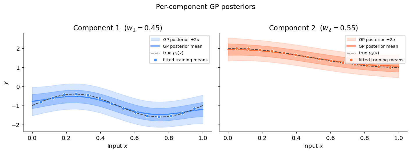
Plot: component GP posteriors

colors_k = [BLUE, ORANGE]
x_plot   = x_pred[:, 0]
x_train_plot = x_train[:, 0]
true_funcs = [mu1, mu2]

fig, axes = plt.subplots(1, K, figsize=(11, 4), sharey=True)

for k, ax in enumerate(axes):
    mu_k  = comp_means[k]
    std_k = comp_stds[k]
    c = colors_k[k]

    ax.fill_between(x_plot, mu_k - 2*std_k, mu_k + 2*std_k,
                    alpha=0.20, color=c, label=r"GP posterior $\pm 2\sigma$")
    ax.fill_between(x_plot, mu_k - std_k, mu_k + std_k,
                    alpha=0.35, color=c)
    ax.plot(x_plot, mu_k, color=c, lw=2, label="GP posterior mean")

    true_mu = true_funcs[k](x_pred)
    ax.plot(x_plot, true_mu, "--", color="#444444", lw=1.4, label=r"true $\mu_k(x)$")

    ax.scatter(x_train_plot, fitted_means[k], s=35, color=c,
               edgecolors="white", linewidths=0.8, zorder=5,
               label="fitted training means")

    ax.set_xlabel("Input $x$")
    if k == 0: ax.set_ylabel("$y$")
    ax.set_title(f"Component {k+1}  ($w_{k+1} = {w_norm[k]:.2f}$)")
    ax.legend(fontsize=8, loc="upper right")

fig.suptitle("Per-component GP posteriors", fontsize=13, y=1.01)
plt.tight_layout(); plt.show()

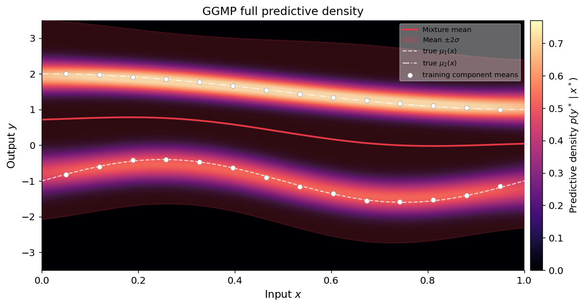
Plot: full predictive density

The heat map shows \(p(y^* \mid x^*)\) across the prediction grid. The two bands correspond to the two mixture components.

fig, ax = plt.subplots(figsize=(10, 5))

pcm = ax.pcolormesh(
    x_pred[:, 0], y_grid, pred_density.T,
    cmap="magma", shading="gouraud",
    vmin=0, vmax=pred_density.max() * 0.95,
)
cb = fig.colorbar(pcm, ax=ax, pad=0.01)
cb.set_label("Predictive density $p(y^* \\mid x^*)$")

ax.plot(x_plot, mix_mean, color=RED, lw=2.0, label="Mixture mean")
ax.fill_between(x_plot, mix_mean - 2*mix_std, mix_mean + 2*mix_std,
                color=RED, alpha=0.20, label=r"Mean $\pm 2\sigma$")

ax.plot(x_plot, mu1(x_pred), "--", color="white", lw=1.2, alpha=0.75, label=r"true $\mu_1(x)$")
ax.plot(x_plot, mu2(x_pred), "-.", color="white", lw=1.2, alpha=0.75, label=r"true $\mu_2(x)$")

ax.scatter(x_train[:, 0], fitted_means[0], s=30, color="white",
           edgecolors="#aaaaaa", linewidths=0.6, zorder=5)
ax.scatter(x_train[:, 0], fitted_means[1], s=30, color="white",
           edgecolors="#aaaaaa", linewidths=0.6, zorder=5,
           label="training component means")

ax.set_xlabel("Input $x$", fontsize=12)
ax.set_ylabel("Output $y$", fontsize=12)
ax.set_title("GGMP full predictive density", fontsize=13)
ax.legend(fontsize=8, loc="upper right", framealpha=0.4)
ax.set_xlim(x_pred[0, 0], x_pred[-1, 0])
ax.set_ylim(y_grid[0], y_grid[-1])
plt.tight_layout(); plt.show()

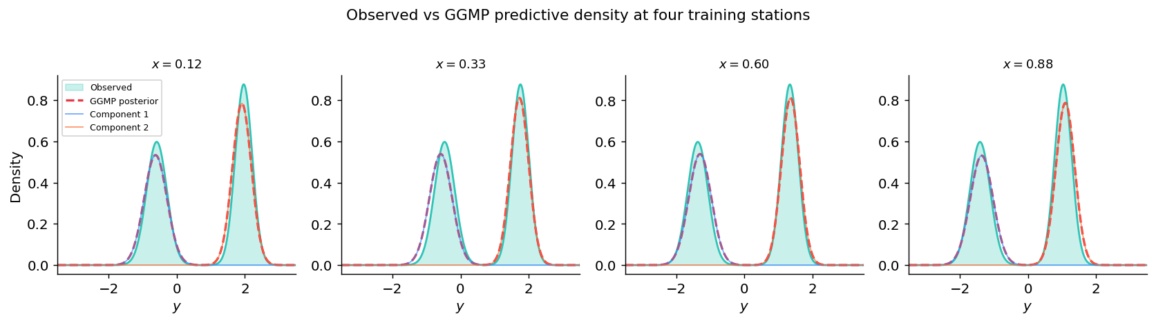
Plot: training data vs posterior side by side

Solid green = observed density at the station; dashed red = GGMP predictive density at the same location.

station_ids = [1, 4, 8, 12]
x_sel = x_train[station_ids]

comp_means_sel = np.stack(
    [g.gps[k].posterior_mean(x_sel)["m(x)"] for k in range(K)], axis=0
)
comp_vars_sel = np.stack(
    [g.gps[k].posterior_covariance(x_sel, variance_only=True)["v(x)"] for k in range(K)], axis=0
)
comp_stds_sel = np.sqrt(np.maximum(comp_vars_sel + mean_noise[:, None], 0))

fig, axes = plt.subplots(1, 4, figsize=(13, 3.5), sharey=False)

for col, (sid, ax) in enumerate(zip(station_ids, axes)):
    xi = float(x_train[sid, 0])
    dom, dens = y_data[sid]
    _, p_obs, _ = ggmp_module._normalize_pdf(dom, dens)

    ax.fill_between(dom, p_obs, alpha=0.25, color=GREEN, label="Observed")
    ax.plot(dom, p_obs, color=GREEN, lw=1.5)

    pred = np.zeros(len(y_grid))
    for k in range(K):
        pred += w_norm[k] * norm.pdf(
            y_grid,
            loc=float(comp_means_sel[k, col]),
            scale=float(comp_stds_sel[k, col]),
        )
    ax.plot(y_grid, pred, "--", color=RED, lw=1.8, label="GGMP posterior")

    for k, c in enumerate(colors_k):
        comp_curve = norm.pdf(
            y_grid,
            loc=float(comp_means_sel[k, col]),
            scale=float(comp_stds_sel[k, col]),
        )
        ax.plot(y_grid, w_norm[k] * comp_curve, color=c, lw=1.0, alpha=0.7,
                label=f"Component {k+1}" if col == 0 else None)

    ax.set_title(f"$x = {xi:.2f}$", fontsize=10)
    ax.set_xlabel("$y$")
    if col == 0:
        ax.set_ylabel("Density")
        ax.legend(fontsize=7)
    ax.set_xlim(dom[0], dom[-1])

fig.suptitle("Observed vs GGMP predictive density at four training stations",
             fontsize=12, y=1.02)
plt.tight_layout(); plt.show()

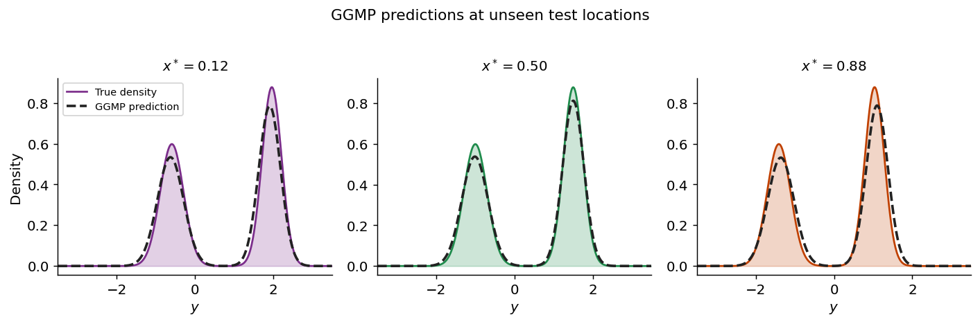
6. Prediction at unseen locations

Three test locations not in the training set — pure generalization.

x_test = np.array([[0.12], [0.50], [0.88]])
labels = [f"$x^* = {xi:.2f}$" for xi in x_test[:, 0]]

comp_means_test = np.stack(
    [g.gps[k].posterior_mean(x_test)["m(x)"] for k in range(K)], axis=0
)
comp_vars_test = np.stack(
    [g.gps[k].posterior_covariance(x_test, variance_only=True)["v(x)"] for k in range(K)], axis=0
)
comp_stds_test = np.sqrt(np.maximum(comp_vars_test + mean_noise[:, None], 0))

def true_density(xi, y):
    return (w_true[0] * norm.pdf(y, float(mu1(xi)), sigma1) +
            w_true[1] * norm.pdf(y, float(mu2(xi)), sigma2))

colors_test = ["#7B2D8B", "#1F8B4C", "#C04000"]
fig, axes = plt.subplots(1, 3, figsize=(11, 3.5))

for col, (xi, ax, lbl, c) in enumerate(
        zip(x_test[:, 0], axes, labels, colors_test)):

    true_dens = true_density(xi, y_grid)
    true_dens /= np.trapezoid(true_dens, y_grid) + 1e-300
    ax.fill_between(y_grid, true_dens, alpha=0.22, color=c)
    ax.plot(y_grid, true_dens, color=c, lw=1.5, label="True density")

    pred = np.zeros(len(y_grid))
    for k in range(K):
        pred += w_norm[k] * norm.pdf(
            y_grid,
            loc=float(comp_means_test[k, col]),
            scale=float(comp_stds_test[k, col]),
        )
    ax.plot(y_grid, pred, "--", color="#222222", lw=2.0, label="GGMP prediction")

    ax.set_title(lbl, fontsize=11)
    ax.set_xlabel("$y$")
    if col == 0:
        ax.set_ylabel("Density")
        ax.legend(fontsize=8)
    ax.set_xlim(y_grid[0], y_grid[-1])

fig.suptitle("GGMP predictions at unseen test locations", fontsize=12, y=1.02)
plt.tight_layout(); plt.show()

Summary

Step	Code
Stage 1 — fit local GMMs	fit_gmm_fixed_weights(samples_n, K, w_init) for each station
Build hyperparameter container	hyperparameters(weights, w_bounds, hps, hps_bounds)
Construct model	GGMP(x_data, y_data, hps_obj=hps_obj, likelihood_terms=K)
Seed likelihoods from Stage 1	g.initLikelihoods(init_mean=..., init_std=..., weights=...)
Build component GPs	g.initGPs()
Stages 2 & 3 — GP hps + weights	g.train(method="local", weight_method="density")
Mixture mean	g.posterior_mean(x_pred)
Mixture variance	g.posterior_variance(x_pred)
Full predictive density	∑_k w_k N(y | μ_k(x*), ν_k(x*) + s̄²_k) per prediction point

Skipping Stage 1 and relying on initLikelihoods()’s default initialization causes the GPs to collapse to constants, because the default uses the bimodal variance (large) as the GP noise. Stage 1 produces the per-component variances that give the GP a realistic noise level.